How to Automatically Number Rows and Cells in Excel: 2 Ways

Numbering rows in Excel sounds like one of those tiny tasks that should take three seconds. Then your worksheet grows to 800 rows, someone deletes row 47, another teammate sorts the data by customer name, and suddenly your neat little list looks like it was organized by a raccoon with a keyboard. The good news: Excel gives you several practical ways to automatically number rows and cells without typing every number by hand.

In this guide, we will focus on two reliable methods: using Excel’s built-in fill tools and using formulas such as ROW and SEQUENCE. These two approaches cover nearly every everyday numbering need, from a quick serial number column to a dynamic list that updates when your data changes.

Whether you are creating an inventory sheet, invoice tracker, classroom gradebook, project list, customer database, or simple to-do list, learning how to automatically number rows and cells in Excel will save time, reduce mistakes, and make your spreadsheets much easier to read.

Why Automatic Numbering in Excel Matters

Excel does not have a single “auto-number this table forever” button in the same way some database tools do. However, it does provide smart features that can create sequential numbers quickly. The best method depends on what kind of worksheet you are building.

If you need a fast, one-time list of numbers, the fill handle or Fill Series tool is perfect. If you need numbers that respond better to sorting, added rows, deleted rows, or changing data ranges, formulas are usually the smarter option. Think of it this way: fill tools are like writing numbers with a very fast pen, while formulas are like hiring a tiny spreadsheet assistant who keeps counting for you.

Method 1: Automatically Number Rows and Cells with Fill Handle or Fill Series

The easiest way to number rows in Excel is to use the Fill Handle. This is the small square at the bottom-right corner of a selected cell or range. Excel can detect a pattern, such as 1, 2, 3, and continue that pattern down a column or across a row.

How to Use the Fill Handle for Sequential Numbering

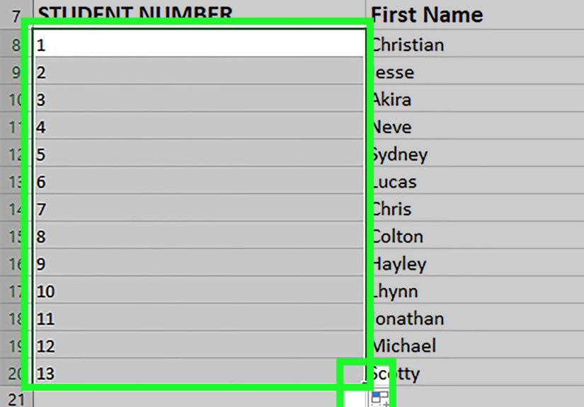
Suppose you want to number a list of products in column A. Your product names begin in column B, starting on row 2. Here is the basic process:

1. Click cell A2 and type 1.
2. Click cell A3 and type 2.
3. Select both cells, A2 and A3.
4. Move your cursor to the small square at the bottom-right corner of the selection.
5. When the cursor changes to a plus sign, drag downward to continue the sequence.

Excel recognizes that you started with 1 and 2, so it continues with 3, 4, 5, and so on. This method works for columns and rows. For example, if you type 1 in B1 and 2 in C1, then drag to the right, Excel can continue numbering horizontally across cells.

Use Double-Click to Fill Faster

If your numbering column is beside a filled data column, you may not even need to drag. Select the first two numbered cells, then double-click the fill handle. Excel will usually fill the sequence down to match the adjacent data range. This is especially useful when you have hundreds or thousands of rows. Dragging through a giant worksheet is nobody’s idea of a thrilling afternoon.

How to Use Fill Series for More Control

The Fill Series command gives you more control than the fill handle. It is useful when you know the exact stopping number or want to create a sequence with a specific step value.

For example, say you want to number cells from 1 to 500 in column A:

1. Type 1 in cell A1.
2. Go to the Home tab.
3. In the Editing group, choose Fill, then Series.
4. Select Columns.
5. Choose Linear.
6. Enter 1 as the Step value.
7. Enter 500 as the Stop value.
8. Click OK.

Excel fills the selected column with a clean sequence from 1 to 500. You can also use a different step value. For example, a step value of 5 creates 1, 6, 11, 16, and so on. If you start with 10 and use a step value of 10, Excel creates 10, 20, 30, 40, and continues from there.

When Method 1 Works Best

The fill handle and Fill Series are best for quick, static numbering. Use this method when your list is mostly finished and you do not expect many row insertions or deletions. It is great for simple checklists, temporary reports, printable sheets, event rosters, or quick data cleanup tasks.

The downside is that filled numbers are static values. If you delete row 6, Excel does not automatically renumber everything below it. If you sort your data incorrectly and do not include the numbering column in the sort range, your numbers may no longer match your records. Static numbering is fast, but it does not think for itself. It is the spreadsheet version of “I did exactly what you asked, not what you meant.”

Method 2: Automatically Number Rows and Cells with Excel Formulas

Formula-based numbering is more flexible. Instead of placing fixed numbers in cells, you use formulas that calculate the number based on row position or data count. The most useful formulas for automatic numbering are ROW and SEQUENCE.

Option A: Use the ROW Function

The ROW function returns the row number of a reference. For example, =ROW(A1) returns 1 because A1 is in the first row. This makes it handy for creating automatic row numbers.

To number a list starting in cell A2, type this formula in A2:

Then copy or drag the formula down. In A2, the formula returns 1. In A3, it becomes =ROW(A2) and returns 2. In A4, it returns 3, and so on.

This approach is useful because the displayed number is based on a formula, not a typed value. If you sort the data properly and include the numbering column with the rest of the table, the formulas can help maintain a logical sequence. If you insert or delete rows, you can usually refresh the formulas by filling them down again or by using them inside an Excel Table.

Number Rows Based on the Current Row Position

If your list starts on row 5 and you want the first item to display as 1, you can subtract the header row position. For example, if your first numbered item is in A5, use:

This formula says, in plain English: “Give me the current row number, then subtract the row number of the header.” Since row 5 minus row 4 equals 1, the first item becomes 1. The next row becomes 2, and the pattern continues.

Use ROW in an Excel Table

For a more dependable setup, convert your data range into an Excel Table. Select your data, press Ctrl + T, confirm the range, and make sure “My table has headers” is checked if you have headers. Excel Tables automatically expand when you add new rows, which makes them useful for ongoing lists.

Inside a table, you can use a formula such as:

This creates a sequence based on the table’s header row. When you add new records at the bottom of the table, Excel can copy the formula down automatically. This is a strong choice for task lists, sales logs, order trackers, and any sheet that keeps growing over time.

Option B: Use the SEQUENCE Function

If you use Excel for Microsoft 365, Excel 2021, Excel 2024, or Excel for the web, the SEQUENCE function is one of the cleanest ways to automatically generate numbers. SEQUENCE creates a dynamic array, meaning the result can spill into multiple cells automatically.

To create numbers 1 through 10, enter:

Excel spills the numbers into 10 rows. You only type one formula, and Excel does the rest. It is neat, fast, and feels slightly like cheating, which is often how good spreadsheet work feels.

The full structure of the SEQUENCE function is:

Here is what each part means:

• rows: how many rows of numbers to generate.
• columns: how many columns to fill.
• start: the first number in the sequence.
• step: the amount to add between numbers.

For example, this formula creates 20 numbers starting at 100 and increasing by 5:

The result is 100, 105, 110, 115, and so on. This is useful for ticket numbers, batch IDs, sample labels, training modules, or any numbering system that does not start at 1.

Number Rows Based on Existing Data with SEQUENCE and COUNTA

One common problem is creating numbering that matches the number of filled records in another column. Suppose column B contains product names, with a header in B1. You want column A to number only the products. You can use:

This counts the non-empty cells in column B, subtracts 1 for the header, and creates a matching sequence. If you add more product names, the numbering can expand automatically, as long as the spill range below the formula is clear.

Be careful with dynamic array formulas inside Excel Tables. SEQUENCE spills into nearby cells, while tables expect formulas to behave row by row. If you get a #SPILL! error, check whether blocked cells or table structure are preventing the formula from expanding.

Which Numbering Method Should You Choose?

Use the fill handle or Fill Series when you want speed. It is the simplest method and works in almost every modern version of Excel. It is also easy to teach to beginners. If someone can drag a corner of a cell, they can number a list.

Use formulas when you want flexibility. The ROW function works well for traditional worksheets and Excel Tables. SEQUENCE is excellent for modern Excel users who want dynamic results with minimal manual work. For growing lists, formula-based numbering usually wins because it reduces maintenance.

A practical rule: if the list will be printed once, use Fill Series. If the list will be edited all month, use a formula. If the list will be edited by five people who all claim they “only changed one tiny thing,” definitely use a formula.

Common Problems and Easy Fixes

The Fill Handle Is Missing

If you do not see the fill handle, it may be disabled. In Excel, go to File, then Options, then Advanced. Look for the setting that enables the fill handle and cell drag-and-drop. Turn it on, then return to your worksheet.

Numbers Repeat Instead of Increasing

If Excel copies 1, 1, 1 instead of creating 1, 2, 3, you probably selected only one starting cell. Type 1 in the first cell and 2 in the next cell, select both, then drag. This gives Excel a pattern to follow.

SEQUENCE Shows a #SPILL! Error

A #SPILL! error usually means the formula wants to place results into multiple cells, but something is blocking the spill range. Clear the cells below or beside the formula. Also check whether merged cells, tables, or hidden content are in the way.

Deleted Rows Break the Numbering

Static numbers from the fill handle will not automatically repair themselves after deleted rows. Use a ROW formula, an Excel Table, or SEQUENCE if you need numbering that is easier to refresh or maintain.

Real-World Examples

Example 1: Inventory List

You manage a small warehouse sheet with item names in column B and categories in column C. If you only need quick serial numbers for a monthly printout, type 1 and 2 in A2 and A3, select both, and double-click the fill handle. Simple, fast, done.

Example 2: Project Tracker

You maintain a project tracker that changes every week. Tasks are added, removed, and sorted by deadline. In this case, use a formula such as =ROW()-ROW($A$1) starting in A2, or convert your range into an Excel Table and use a table-friendly ROW formula. Your future self will silently thank you.

Example 3: Training Attendance Sheet

You have a training attendance sheet where names are added over time. If your names are in column B, you can use =SEQUENCE(COUNTA(B:B)-1) in A2. As the list grows, the numbering can expand automatically, provided the spill area stays empty.

Extra Experience: Practical Lessons from Automatically Numbering Rows and Cells in Excel

After working with many Excel sheets, one lesson becomes obvious: numbering looks simple until the worksheet becomes important. A plain serial number column can affect filtering, sorting, printing, auditing, and communication. When a manager says, “Check item 138,” everyone needs item 138 to actually be item 138. If your numbering is broken, the conversation quickly turns into a spreadsheet treasure hunt.

One practical habit is to decide whether the number is just a visual row label or a permanent record ID. A visual row label can change when rows are sorted or deleted. For that, ROW or SEQUENCE works well. A permanent record ID should not change after it is assigned. For example, invoice number 1025 should remain invoice number 1025 even if you sort invoices by customer name. In that situation, you may want static values, controlled ID rules, or even a database system rather than a simple row formula.

Another experience-based tip is to keep numbering formulas away from messy data when possible. If you use COUNTA(B:B), remember that any extra text in column B can affect the count. A forgotten note at the bottom of the sheet may make your sequence longer than expected. For cleaner results, use a specific range such as B2:B500 instead of the entire column when your worksheet has notes, totals, or instructions below the main data.

Excel Tables are especially useful for long-term worksheets. They make formulas easier to maintain, expand automatically, and keep filters organized. However, dynamic array formulas like SEQUENCE may not behave the same way inside tables because spilled arrays need free space. If you are using a table, ROW-based formulas are often more predictable. If you are using a normal range in modern Excel, SEQUENCE is beautifully efficient.

It is also smart to protect formulas when sharing a workbook. Many numbering problems happen because someone accidentally types over a formula in the middle of the list. If the sheet is used by a team, consider locking formula cells or keeping a backup copy. You can also use a clear header such as “Auto No.” or “Do Not Edit” if your coworkers are known to treat spreadsheets like a contact sport.

Finally, test your numbering method before trusting it. Insert a row. Delete a row. Sort the data. Filter the data. Add a new record at the bottom. If the numbering still behaves the way you want, you have chosen the right method. A five-minute test can prevent a two-hour cleanup later. Excel is powerful, but it appreciates a little supervisionlike a smart intern who occasionally needs coffee and boundaries.

Conclusion

Learning how to automatically number rows and cells in Excel is one of those small skills that pays off again and again. For quick lists, the fill handle and Fill Series command are fast and beginner-friendly. For flexible worksheets, formulas like ROW and SEQUENCE are more powerful because they can adapt better to changing data.

The best approach depends on your goal. Use static numbering for simple, finished lists. Use formula-based numbering for living worksheets that will be edited, sorted, expanded, or shared. Once you understand both methods, you can stop typing numbers manually and let Excel handle the boring part. Your keyboard, your patience, and your future spreadsheet cleanup schedule will all be grateful.