How to Use AutoFilter in MS Excel: A Step-by-Step Guide

If you have ever opened a spreadsheet and felt like the data was staring back at you like a wall of tiny, judgmental rectangles, AutoFilter is here to help. This built-in Excel feature lets you show only the rows you need while hiding the rest, which is a polite way of saying it helps you stop scrolling forever. Whether you are sorting through sales reports, customer lists, inventory sheets, or a class gradebook, AutoFilter can turn spreadsheet chaos into something that actually makes sense.

In this guide, you will learn exactly how to use AutoFilter in MS Excel step by step. We will cover the setup, the filtering options, the common mistakes, and the little tricks that make the feature much more powerful than most people realize. By the end, you will be able to filter text, numbers, dates, colors, and multiple columns like someone who definitely reads spreadsheets for fun.

What Is AutoFilter in MS Excel?

AutoFilter is Excel’s built-in filtering tool that adds drop-down arrows to your header row. Those arrows let you quickly narrow down a list based on criteria such as names, values, dates, colors, or specific keywords. Instead of deleting rows or creating a bunch of duplicate sheets, AutoFilter simply hides what does not match your conditions.

That means your original data stays intact. You are not changing the list itself. You are just changing what is visible on screen. That is a huge deal when you need to review records without wrecking your worksheet like a raccoon in a snack drawer.

Why AutoFilter Is So Useful

AutoFilter saves time, reduces mistakes, and makes large worksheets easier to understand. If you have 5,000 rows of transactions and only want to see orders from Texas in January over $500, AutoFilter can pull that off in seconds. It is also great when you want to review blanks, find duplicates visually, isolate specific departments, or troubleshoot bad entries without manually hunting down every row.

For beginners, the best part is that AutoFilter does not require formulas. For advanced users, the best part is that it still works beautifully even when your data gets messy, large, and annoyingly human.

Before You Start Filtering

Before you turn on AutoFilter, take two minutes to set up your worksheet properly. This is the part people skip right before asking why Excel is “broken.” Usually, Excel is fine. It is just being literal.

1. Make Sure Your Data Has Headers

Each column should have a clear label in the first row, such as Name, Region, Order Date, or Revenue. AutoFilter uses these headers for the drop-down menus.

2. Remove Blank Rows and Blank Columns

Blank rows can interrupt your data range and prevent Excel from filtering the full list. If your table has random empty lines in the middle, clean them up first.

3. Keep Data Types Consistent

Try not to mix numbers with text in the same column. A column with dates should contain dates. A column with prices should contain numbers. If one row says 1250 and another says one thousand two hundred fifty, Excel will not magically decide those are the same thing.

4. Consider Converting the Range to a Table

Excel tables are especially filter-friendly. They automatically include header filters, expand when new rows are added, and make ongoing data management much easier. If you work with the list regularly, turning it into a table is often the smartest move.

How to Use AutoFilter in MS Excel: Step by Step

Step 1: Select Your Data Range

Click anywhere inside your dataset. You do not always need to highlight the whole range manually. If your data is organized properly, Excel can usually detect the list on its own. Still, if the dataset is messy, selecting the full range yourself can prevent surprises.

Example: Suppose you have columns for Employee Name, Department, Hire Date, and Salary. Click any cell inside that block of data.

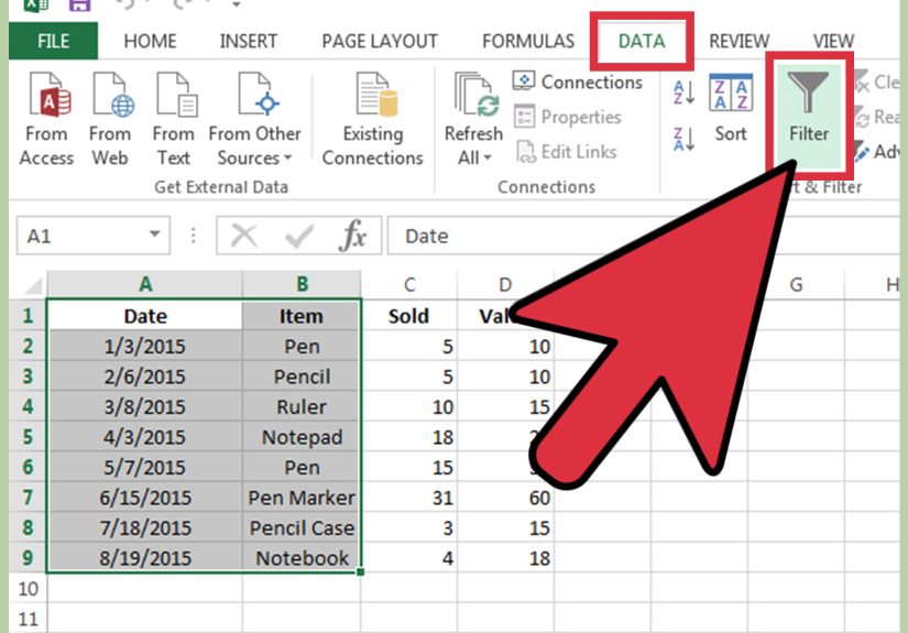
Step 2: Turn On AutoFilter

Go to the Data tab on the ribbon and click Filter. Instantly, little drop-down arrows will appear in the header row. Congratulations, you are now in filtering territory.

A handy shortcut is Ctrl + Shift + L, which toggles AutoFilter on and off. It is fast, satisfying, and makes you look like the person who knows what they are doing.

Step 3: Filter by Specific Values

Click the drop-down arrow in the column you want to filter. You will see a checklist of values from that column. Uncheck Select All, then check only the items you want to display.

Example: In a Department column, you might select only Marketing and Sales. Excel will hide the rest of the rows automatically.

This is one of the quickest ways to isolate categories, regions, product types, or status labels.

Step 4: Use the Search Box Inside the Filter Menu

If the column contains a long list of entries, use the search box at the top of the filter menu. Type part of a value and Excel will narrow the checklist for you.

Example: In a customer list, typing smith can help you find every matching entry without scrolling through 1,200 names and questioning your career choices.

Step 5: Apply Text Filters

For columns containing text, Excel offers options like Equals, Does Not Equal, Begins With, Ends With, and Contains. These are perfect when you need more precision than a simple checkbox list.

Example: In a City column, choose Text Filters > Begins With and enter San. That can show San Diego, San Jose, and San Antonio in one shot.

This is especially useful for messy lists where categories are not standardized perfectly.

Step 6: Apply Number Filters

If the column contains numbers, you can use filters like Greater Than, Less Than, Between, Top 10, or Above Average.

Example: In a Revenue column, choose Number Filters > Greater Than and enter 1000. Excel will show only rows where revenue exceeds that amount.

This is fantastic for sales analysis, budget tracking, performance reviews, and finding out which products are actually carrying the team.

Step 7: Filter Dates

Date columns are even more powerful because Excel groups them by year, month, and day. You can filter by a specific month, a custom date range, or relative options such as last month or next quarter, depending on the version and context.

Example: In an Order Date column, you can show only records from March 2026 or filter to dates between January 1 and March 31.

When date filtering seems weird, the usual culprit is that the “dates” are actually text. If Excel does not recognize them as real dates, the date filter options will not behave properly.

Step 8: Filter by Color or Icon

If your worksheet uses cell fill colors, font colors, or icon sets from conditional formatting, AutoFilter can filter by those too.

Example: If overdue tasks are highlighted in red, you can filter by red cell color to show only the urgent items. Suddenly, your sheet becomes a to-do list with a pulse.

This is a practical way to review flagged items without creating another helper column.

Step 9: Filter Multiple Columns at Once

AutoFilter becomes much more powerful when you combine filters across columns. Excel applies them together, so each new filter narrows the visible list further.

Example: You can filter a sales sheet to show:

• Region = West
• Product Category = Office Supplies
• Revenue > 500
• Order Date = February 2026

That kind of multi-column filtering is where Excel stops being just a spreadsheet and starts acting like a lightweight database.

Step 10: Clear, Reapply, or Remove Filters

When you are done, you have a few options:

• Clear one filter by opening that column’s drop-down and choosing Clear Filter.
• Clear all filters from the sheet using the ribbon’s sort and filter controls.
• Turn AutoFilter off entirely by clicking Data > Filter again or pressing Ctrl + Shift + L.
• Reapply filters after data changes if the current view needs refreshing.

This matters because filtered views do not always update automatically when you edit underlying values. If the results look off, a reapply action usually fixes it.

Common AutoFilter Mistakes and How to Fix Them

Headers Are Missing or Incorrect

If Excel thinks your first data row is a header, filtering gets ugly fast. Make sure the top row contains true labels and not actual records.

Numbers or Dates Are Stored as Text

If number filters or date filters are unavailable, Excel may be reading those entries as text. Convert the values properly before filtering.

Blank Rows Break the Range

One empty row in the middle of your list can cause Excel to filter only part of the dataset. Delete blank rows before you begin.

Not All Columns Were Included

If you turn on AutoFilter for only one section of the data, related columns may stay unfiltered. Always confirm the full dataset is included.

Hidden Rows Are Confusing the View

Manual hidden rows and filtered rows are not the same thing. If the sheet looks incomplete, check whether some rows were hidden manually before the filter was applied.

AutoFilter vs. the FILTER Function

This confuses a lot of Excel users, so let’s clear it up. AutoFilter is the drop-down feature built into column headers that hides nonmatching rows in place. The FILTER function is a formula that returns matching data into another range.

Use AutoFilter when you want to work directly inside the original dataset. Use the FILTER function when you want a separate dynamic result elsewhere in the sheet. One is interactive. The other is formula-driven. Both are useful. They are cousins, not twins.

Helpful Tips for Using AutoFilter More Efficiently

• Use keyboard shortcuts: Ctrl + Shift + L toggles filters, and Alt + Down Arrow opens a header menu quickly.
• Format data as a table: Tables keep filters attached as your data grows.
• Use consistent naming: Clean category labels make filtering more reliable.
• Add helper columns when needed: If your logic is complicated, helper columns can simplify the filter criteria.
• Combine filtering with sorting: Filter first, then sort the visible results to surface patterns faster.

Real-World Example of AutoFilter in Excel

Imagine you manage an online store and your worksheet tracks thousands of orders. The columns include Order ID, Customer Name, State, Order Date, Status, and Total. Your boss asks for all California orders from March that are Pending and worth more than $200.

Instead of creating a new file, manually copying rows, or pretending your Wi-Fi went out, you can use AutoFilter:

1. Turn on AutoFilter.
2. Filter State to California.
3. Filter Order Date to March.
4. Filter Status to Pending.
5. Filter Total to values greater than 200.

Done. Clean, fast, and far less dramatic than most spreadsheet emergencies.

Conclusion

Learning how to use AutoFilter in MS Excel is one of the simplest ways to get more control over your data. It helps you focus on the rows that matter, speeds up analysis, and makes even large worksheets feel manageable. Once you know how to filter by text, number, date, color, and multiple columns, you can work faster without touching a single advanced formula.

The best part is that AutoFilter is useful whether you are a beginner organizing a class project or a professional reviewing thousands of records. It is one of those Excel features that looks small until you start using it every day. Then suddenly it becomes the office hero you did not know you needed.

Experience and Practical Lessons From Using AutoFilter in Real Work

One of the biggest lessons people learn with AutoFilter is that the feature feels almost too simple at first. You click a button, choose a few values, and rows disappear. Nice. Helpful. Maybe even mildly exciting if you are the sort of person who finds satisfaction in a well-behaved spreadsheet. But after using AutoFilter in real work, you realize it is not just a convenience tool. It changes how you think about large lists.

For example, many beginners start by scrolling through data manually. They search with their eyes, which is a noble effort but a terrible long-term strategy. In a worksheet with a few dozen rows, that works. In a worksheet with a few thousand, it becomes a slow-motion tragedy. AutoFilter teaches you to stop looking at everything and start asking better questions. Show me only late invoices. Show me only East Coast customers. Show me only items below reorder level. That shift is incredibly useful.

Another real-world experience is discovering how much clean data matters. AutoFilter is powerful, but it does not perform miracles. If one department name is entered as HR, another as Human Resources, and another as human resources with a sneaky extra space at the end, your filter results will reflect that mess. Many users do not realize that AutoFilter becomes dramatically better when the source data is standardized. In other words, the feature rewards good habits.

AutoFilter is also surprisingly helpful during error checking. If you suspect a column has blanks where values should exist, filter blanks. If you think someone entered a future date by mistake, filter the date column. If a budget sheet seems off, filter to the highest values first. Instead of scanning row by row, you let Excel pull the suspicious records to the surface. It feels less like hunting and more like using a flashlight.

In team settings, AutoFilter becomes even more valuable because it helps people answer quick questions without altering shared data. A manager can filter by region. An accountant can filter by amount. A coordinator can filter by status. Everyone can investigate the same worksheet from a different angle without duplicating files all over the place like digital confetti.

Perhaps the most underrated experience is confidence. Once users understand AutoFilter, large spreadsheets stop feeling intimidating. The data is still large, yes, but it no longer feels untouchable. You know you can narrow it, sort it, search it, and reshape the view in seconds. That confidence tends to lead to better analysis, fewer manual mistakes, and much less spreadsheet panic before meetings.

So while AutoFilter may not have the glamour of a dashboard or the drama of a complex nested formula, it is often the feature people end up using the most. Quietly. Constantly. Reliably. Like a good office coffee machine, only with fewer grounds and better logic.